Knot so easy: Mathematical Proofs from High-performance Solvers?
Computers are able to solve an increasing range of problems, many of which were believed not long ago to require human intelligence. Yet there are fundamental limitations to what problems can be solved algorithmically, some known and other conjectured. In particular, by results of Gödel, Turing, Church and others, there is no computer program that, given a mathematical statement as input, either gives a proof or (correctly) says that the statement is false.
Indeed, we cannot algorithmically solve even a seemingly simple class of problems: deciding whether a so called Diophantine Equation, has a solution. A Diophantine equation is a polynomial equation with integer coefficients, such as $3n^2 + 7m^2 = r^3$, with solutions being integers corresponding to the variables ($n$,$m$ and $r$ in the example) which satisfy the equation. For instance, we say that the Diophantine equation $n^2 = 2$ has no solution even though $n= \sqrt{2}$ is a solution over real numbers, as $n$ is required to be an integer in a Diophantine solution. As a result of combined work of Martin Davis, Yuri Matiyasevich, Hilary Putnam and Julia Robinson during the 1950s and 1960s, we know that there is no algorithm (i.e., computer program) to which we can input the coefficients of a Diophantine equation and which will tell us (correctly) whether the equation has integral solutions.
Yet, the above results should not be over-interpreted to say that proofs cannot be found by programs. Indeed if we turn from numbers to the other classical source of mathematics – Euclidean geometry, the situation is different. In the 1950s, Tarski proved that whether a (finite) collection of polynomial equations and inequations has solutions that are real numbers is decidable. Using coordinate geometry, statements in Euclidean geometry can be translated to such problems, and so are algorithmically decidable. Tarski’s algorithm has been greatly improved, and algorithms of a more algebraic nature have also been developed, improved and implemented. Yet they remain slow.
This post is about by my experiments to use (as an amateur) state-of-the-art solvers to try in practice to prove such results and other related stuff. I started these experiments prompted by a lecture to undergraduate students, during which I used Z3, a high-performance solver from Microsoft, to solve a Sudoku problem (a standard demo for this technology). The puzzle was duly solved instantly. You can see such a demo online, but the online version is slow.
I looked around for examples of geometric theorems proved using Z3 or its friends, but found none. So I decided to try my hands at proving some results in this way. I also redid experiments I had tried some years ago, using Z3 for recognizing knotting, using an algorithm which follows essentially immediately from a result of Kronheimer-Mrowka.
Unfortunately, at least in the way I used them, neither Z3 nor CVC4 (another similar system, and the champion in the latest SMT prover competition) failed to prove the geometric result I sought. Yet, especially as these systems are vastly improving, it seems worthwhile to write about how such systems can be used at least in principle, especially since this does not seem to be widely known.
P versus NP and SAT/SMT solvers
Some problems, such as solving a system of linear equations, are not difficult, at least once one knows a method to solve them. The thumb rule used is that if we can solve a problem with the number of steps being at most a polynomial in the size of the problem (for instance, the total number of digits in the coefficients of equations), then we consider the problem to be easy enough. The class of these problems is called $P$ (i.e., Polynomial time).
A more interesting class of problems is ones for which we can check that a solution is correct reasonably easily, though it may not be clear how to find a solution in an easy manner. This is typically the case with puzzles like jigsaws or Sudoku — indeed the appeal of puzzles perhaps lies in this feature. Such problems are called $NP$ problems (or problems in the class $NP$). While it appears that many such problems do not have easy (i.e., polynomial time) solutions, there is no proof of this. Whether every problem whose solution is easy to check has a solution that is easy to find is the $P$ versus $NP$ problem.
What makes this problem specially interesting and fruitful is the Cook-Levine theorem from the early 1970s. This says that if one specific problem in NP, called the Boolean satisfiability problem (or $SAT$), has a polynomial time solution, then every problem that is in $NP$ can be solved in polynomial time. It can be deduced that there are many other problems with the same property. Such problems are called $NP$-complete.
SAT solvers
While the theoretical $P$ vs $NP$ problem remains mysterious, the Cook-Levine theorem has had some remarkable practical uses. Since so many classes of problems can be reduced to solving one class of problems, namely $SAT$, a powerful approach has been to develop various clever ways, and powerful programs incorporating them, to solve $SAT$ problems better, and then using these to solve other problems. Such programs are called $SAT$ solvers .
More precisely, the Boolean satisfiability problem ($SAT$), like the solvability of Diophantine equations, asks whether a set of equations has a solution (sets of equations having solutions are said to be satisfiable). However these are equations with variables representing not integers or reals but so called Booleans, i.e., which can be either $\textrm{true}$ or $\textrm{false}$. From such variables we build statements using the logical operations and, or and not. For example, for Boolean variables $P$ and $Q$, we may require than $P$ is $\textrm{true}$ and $Q$ is false, i.e., $\textrm{not}\ Q$ (denoted $\neg Q$) is $\textrm{true}$. Given a finite list of such conditions, we may or may not have a solution — for example $P$ being true and $P$ being false cannot both be satisfied. Determining whether there is a solution to a finite list of Boolean statements is the problem $SAT$. Clearly given a solution it is easy to check that it is correct, so $SAT$ is in $NP$.
While it appears that no program can solve all $SAT$ problems reasonably fast (i.e., in polynomial time), high-performance $SAT$ solvers try to solve as large a class of $SAT$ problems as quickly as possible in practice. Indeed in many cases $SAT$ problems are not that hard — for example the problem becomes easier if there are either so many solutions that one can readily find one or so many constraints that one can readily show that there are none.
$SMT$ solvers (for Satisfiability Modulo Theories) extend these ideas to handle problems that involve not just Booleans, but also integers and real numbers. Thus, we can require that a collection of equations are satisfied, or a mixture of equations and inequations (inequations can be like $x^2 < 3$, $x^3 \geq 3z$ or $y^2 + z^2 \neq 1$) or even a logical combination of these (e.g. ($x^2 < 3)\vee(y^2 + z^2 \neq 1)$, where $\vee$ is the logical or). Again, many instances of these problems are hard, and there are even ones with no algorithmic solution. Nevertheless the approach taken is to solve as large a class of problems as efficiently as possible.
Pappus hexagon theorem: attempting geometry
In principle SMT solvers can be used to solve problems in Euclidean geometry. I attempted to prove the Pappus hexagon theorem, which I next describe. In addition to being a typical geometry result, this has a deeper mathematical meaning (corresponding to commutativity for affine geometries over division rings).
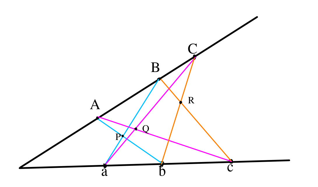
Suppose we are given two lines, with points $a$, $b$ and $c$ on the first line and $A$, $B$ and $C$ on the second line as in the figure below. We consider the general case, where no pair of lines involving these points are parallel. Let $P$ be the intersection of the lines $Ab$ and $aB$, $Q$ the intersection of $Ac$ and $aC$, and $R$ the intersection of $Bc$ and $bC$. The Pappus hexagon theorem is the result that $P$, $Q$ and $R$ are collinear, i.e., there is a line containing all three of these points, for all choices of $a$, $b$, $c$, $A$, $B$, and $C$ of the above form.
Equations for collinearity
We shall translate this into a problem of deciding whether a collection of polynomial equation and inequations over reals has a solution, which as Tarski showed is decidable. First, we recall that collinearity can be expressed as a polynomial equality. Namely,
points with coordinates $(x_1, y_1)$, $(x_2, y_2)$ and $(x_3, y_3)$, which we assume to be distinct, are collinear if and only if
$$\frac{y_2 - y_1}{x_2 - x_1} = \frac{y_3 - y_1}{x_3 - x_1}$$
which is equivalent to $$(y_2 - y_1)(x_3 - x_1) = (y_3 - y_1)(x_2 - x_1).$$
A simple problem
As a warmup and sanity check, I set up the problem of showing that for an arbitrary point $P = (x, y)$, the three points $P=(x, y)$, $O=(0, 0)$ and $-P=(-x, -y)$ are collinear.
We prove such results using SMT solvers by contradiction. In this case, for variables $x$ and $y$, we impose the condition that the points $P$, $O$ and $-P$ are not collinear. If the solver shows that this cannot be satisfied, then it follows that the points are always collinear. Observe that the condition of not being collinear just means that equation in the above equation is replaced by the inequation $(y_2 - y_1)(x_3 - x_1) \neq (y_3 - y_1)(x_2 - x_1)$.
Indeed the solvers Z3 and CVC4 prove this result instantly — more precisely, Z3 took $0.012$ seconds and CVC4 took $0.094$ seconds.
Choosing coordinates
While one can (and I initially did) take arbitrary coordinates for the $6$ points $a$, $b$, $c$, $A$, $B$ and $C$ and add equations for their being collinear, we consider a simpler variant where we choose coordinates and parametrize the points. Namely, we can take $a$, $b$ and $c$ on the x-axis with $a = (1, 0)$. Then we have $b = (1 + u, 0)$ and $c = (1 + u + v, 0)$ with $u>0$ and $v>0$. Similarly, if we let $A = (x_A, y_A)$, then we can assume that $B = (x_A(1+ U), y_A(1 + U))$ for some $U > 0$ and $C = (x_A(1+ U + V), y_A(1 + U + V))$ for some $V > 0$. Further, we can assume that $y_A > 0$.
Let the points $P= (x_P, y_p)$, $Q = (x_Q, y_Q)$ and $R= (x_R, y_R)$ have arbitrary coordinates. We add equations corresponding to their being intersection points as we see below. Thus, we have $12$ variables in all, $6$ of them the parameters $u$, $v$, $x_A$, $y_A$, $U$ and $V$ for the problem and $6$ more coordinates of the intersection points. Further, we have inequations $u >0$, $v >0$, $y_A >0$, $U > 0$ and $V >0$. We shall add to these equations and inequations from the statement of the theorem.
Formulating using polynomial equations and inequations
We reformulate the Pappus hexagon theorem in terms of collinearity. Observe that $P$ being the intersection point of $Ab$ and $aC$ is equivalent to both the triples of points $(A, P, b)$ and $(a, P, B)$ being collinear. We have similar conditions for $Q$ and $R$. Thus, the conditions on $P$, $Q$ and $R$ can be formulated in terms of collinearity of $6$ triples of points.
Finally, the conclusion is that $P$, $Q$ and $R$ are collinear. We seek to prove this by contradiction, namely we add the condition that they are not collinear, and show that the resulting system cannot be satisfied. Again, the condition that the points are not collinear gives an inequation.
In summary, we have a problem asking whether a set of algebraic equations and inequations has a solution over reals. This system has $12$ variables, with $6$ equations corresponding to collinearity, $5$ inequations stating that variables are positive and an inequation (to contradict) stating that three points are not collinear.
Running SMT solvers
As mentioned in the introduction, neither of the SMT solvers was able to prove the Pappus hexagon theorem. This was in spite of my (undoubtedly amateur) attempts at changing their parameters to raise various limits.
To try to assess how far they were from proving the theorem, I attempted a simpler variant. Instead of having all six of $u$, $v$, $x_A$, $y_A$, $U$ and $V$ as variables (so proving the result for all values of these), I added additional equations fixing some of them. Since all but $x_A$ were known to be positive, for convenience, conditions could only be added by choosing random positive numbers corresponding to some of the five variables $u$, $v$, $y_A$, $U$ and $V$ and adding corresponding equations — for example, we could pick $c > 0$ at random and add the equation $u = c$.
When all $5$ of the variables were fixed (leaving only $x_A$ to vary), Z3 solved the problem instantly. When $4$ of the $5$ were fixed, the theorem was proved in about 6 seconds. However, when only $3$ were fixed I could not get either solver to prove the result, in spite of changing parameters.
Knot so easy
A related attempt (with common code) concerned an algorithmic problem in topology. A basic decision problem in topology is the unknotting problem, which is deciding whether a smooth embedding $K$ of the circle into $\R^3$ is the boundary of a smooth embedding of a disc. We say $K$ is unknotted if it bounds a smoothly embedded disc. An algorithm to solve the decision problem was found in the 1950s by Haken. However, Haken’s algorithm was doubly exponential, and so not practical.
As had been independently observed by many people, there is another kind of algorithm that follows immediately from some deep work of Kronheimer-Mrowka where they proved what was called Property P, a baby version of the Poincaré conjecture (Perelman proved the Poincaré conjecture itself some years after this work of Kronheimer-Mrowka).
Unknotting and Groups
It has been known from the 1950s that the knotting problem is equivalent to whether the so called Knot Group $G_K$ associated to a knot $K$ is isomorphic to the integers. However deciding whether groups are isomorphic, or even whether a group is non-trivial, are algorithmically undecidable. What Kronheimer-Mrowka showed was that a certain quotient $\overline{G}_K$ of $G_K$ is the trivial group if and only if $K$ is unknotted ($\overline{G}_K$ is the fundamental group of the manifold obtained by $+1$ surgery about the knot `$K$).
This criterion does not give an algorithm as we cannot decide whether a group is trivial (as mentioned above). However, Kronheimer-Mrowka proved more, namely if $K$ is not unknotted, then $\overline{G}_K$ has a non-trivial homomorphism into $SU(2)$, the group of unit quaternions. The existence of such homomorphisms is indeed decidable, as we sketch in the next section (requiring more of a mathematical background than the preceding).
Deciding existence of non-trivial homomorphisms
Just as complex numbers $z = x + iy$ correspond to pairs of real numbers, quaternions are numbers $z = a + bi + cj+ dk$ corresponding $4$ real numbers, with $i$, $j$ and $k$ special quaternions. Unit quaternions are those that satisfy $a^2+ b^2 + c^2+d^2=1$. These can be multiplied, and form the group $SU(2)$. Note that since we consider unit quaternions, inversion is just conjugation, so linear in terms of the coefficients.
Given a presentation of a group G=$\langle \alpha_1, \dots, \alpha_n; r_1, \dots,r_m \rangle$, a homomorphism from $\rho:G \to SU(2)$ is determined by the images of the generators, which are determined by the $4$ components of quaternions. Thus, we have $4n$ variables. These satisfy two kinds of equations. Firstly, the images being unit quaternions gives an equation for each generator. On the other hand, the coefficients of $\rho(\alpha_i)$ for the generators $\alpha_i$ determine coefficients of the images $\rho(r_j)$ of the relations. A necessary and sufficient condition for $\rho$ to be a homomorphism is that these are all the identity. This gives the second set of equations. Finally non-triviality is the condition that the image of some generator is not the identity.
Thus, given a presentation of a group $G$, we get an SMT problem corresponding to $G$ having a non-trivial homomorphism to $SU(2)$. I implemented the translation and tried this for a few presentations of groups. Once more, my success was limited. For simple presentations I easily obtained either non-trivial homomorphisms or a proof of non-existence of these. However the solvers quickly reached their limits.
I must mention that now there is now a practical solution of the unknotting problem, again due to Kronheimer-Mrowka, based on a characterization in terms of Khovanov homology.
Final remarks
The negative results at least show that, at present, we cannot hope to solve non-trivial Euclidean geometry questions by simply translating them and using SMT solvers, as also for problems that translate to matrix equations. However, with the underlying solvers rapidly improving, the solutions in principle may become solutions in practice. This is especially the case if the algorithms are successfully parallelized — to my surprise I observed that the algorithms were essentially serial even when configured to be parallel, with occasional use of $2$ cores being the only concurrency.
It would also be interesting to see in greater detail what causes such algorithms to be so slow, say with the above model problems. In particular, while it is known that in the worst case any algorithm must be slow, perhaps there are special features in cases of interest that allow speeding up.